Introduction
I contend that no college football fanbase has a more unfortunate balance of perceived potential of their team vs the actual performance on the field than the University of Michigan. Though the message board posts on the most prominent Michigan sports blog, MGoBlog, have had a decidedly pessimistic tone for the past couple years, I don’t know a Michigan fan alive who doesn’t truly believe that the Wolverines have a legitimate shot at winning a game once the shoe meets the leather on game day.
I, unfortunately, am not immune to this affliction. I’m acutely aware of all the shortcomings of our roster. I know that our quarterbacks don’t see the wide open guy a lot of the time. I’ve spent countless hours reading MGoBlog threads about why our defensive line is so thin. And yet, at kickoff these thoughts leave my head, replaced by the thought that we should win no matter what.
That’s a long winded way of saying that Michigan fans (myself included) can get a little carried away with analyzing the minutia of the game. This is where my computer vision project starts. After a particularly demoralizing game (a win, oddly enough) against Army, I decided to work on a project that takes a game broadcast as an input and output analytics about offensive tendencies. The goal is to eventually be able to predict the plays and formations that a team might choose based on features like down, distance, field position, score, etc. I’m not quite there yet, but I figured I should write up what I have so far.
What I Have So Far
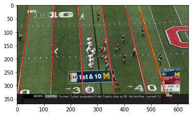
The problem I’ve been working on solving is the very first one: given footage of an entire game broadcast, how do you identify the important frames? In other words, without watching the footage, how do you know which frames are the “presnap” frames? Presnap frames are the frames of the video taken just before a play starts. These selected frames have the contextual information we’re after: the down, distance, and score, but most importantly the formation that the offense is using. Down the line I’ll add outcome (yards gained/lost, was it a scoring play) and play (run v pass, what kind of run or pass, etc). For now, teaching a computer the difference between presnap and nonpresnap frames is enough of a challenge.
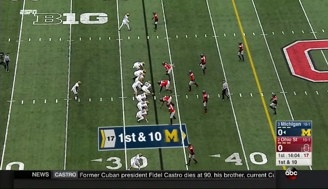
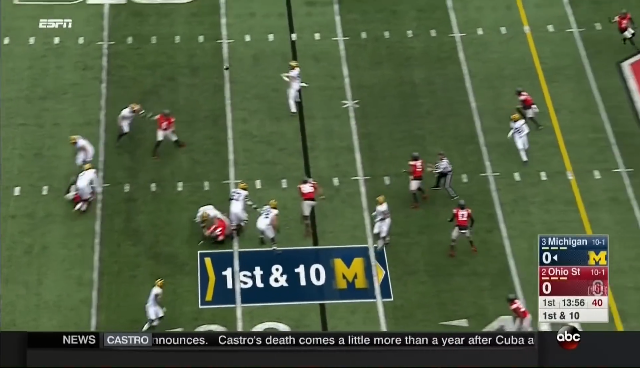
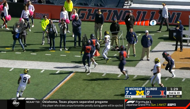
Above is an example of a presnap and a couple nonpresnap frames. The first question to answer is what are a few characteristics I can use to distinguish between these classes of photos? The features that I came up with were:
- number of lines – all presnap images should have yard line markers present, but not all nonpresnap images will
- dominant color – most presnap images will likely have a shade of green as the most prominent color
- blur – presnap images are less blurry than postsnap images
- count of people – as the play starts, the camera shifts focus from all players to the player with the ball
- position of people – presnap images begin with people centered in the frame. As the play progresses, people distribute throughout the frame.
Another feature that I ended up putting in the model is a Principal Component Analysis (PCA) that outputs 5 features. PCA is a process that allows large datasets to be expressed in just a few terms that capture the relationship between the data. In my case, I’m pulling out just the top 5 principal components. I found this resource to be immensely helpful in gaining a basic understanding of the process.
In testing out these features, I found that a combination of dominant color, blur, PCA, and lines gave me the best results. I’ll focus on these features specifically.
Image Processing
Reading in an Image
The first step in doing any sort of work on an image in Python is to read in the image. For this I’m using the cv2 library aka opencv, which I use for a lot of the image manipulation in this project.
import cv2

img_pth = '../presnap_example_raw.png'

img_bgr = cv2.imread(img_pth)
img_rgb = cv2.cvtColor(img_bgr, cv2.COLOR_BGR2RGB)
img_rgb = cv2.resize(img_rgb, (640, 368))

img_grayscale = cv2.cvtColor(img_rgb, cv2.COLOR_RGB2GRAY)
Your image has been read in as a numpy array of the shape (image height x image weight x 3). Each pixel is represented by its RGB values. You’ll notice above that I’m reading in the file, but also converting the color and resizing the image. cv2 reads images in using the BGR image format, but I like working off grayscale and RGB images as they’re easier to view.
Flattening the Image
For the PCA component, we’ll need to change the image into a long 1D array. Luckily numpy makes this easy on us.
flattened_img = img_rgb.flatten()And that’s it! You’re done. You read in the image, you resized it, and now you have an RGB, grayscale, and flattened versions.
Extracting Features
Number of Lines
Above is what I mean by the number of lines in the frame. I won’t get into all the mechanics, mostly because other resources explain it far better than I can. We’re using OpenCV’s Hough Line Transform function to extract lines from a frame, then filtering out non vertical or duplicate lines, and then returning the counts.
We’ll use the grayscale image for this feature. The first step is to apply a Gaussian blur, which helps smooth out edges a bit.
gaussianblur_img = cv2.GaussianBlur(img_grayscale, (5, 5), 0)Next, we’ll do our edge detection with Canny. This process transforms our gray scale image into a series of edges, making the vertical lines we’re after much easier to detect.
def calculateCannyThresholds(image, sigma=0.33):
    std = np.std(image)
    _75thPctlPixelIntensity = np.percentile(image, 75)

    lower = int(max(185, _75thPctlPixelIntensity + (std / 2.0)))
    upper = int(min(240, _75thPctlPixelIntensity + (2.0 * std)))

    return [lower, upper]

def applyCannyEdges(gaussianImg, autoThresholds=True, low_threshold=200, high_threshold=300):
    '''Apply the Canny Edges algorithm to the image'''
    if autoThresholds is True:
        low_threshold, high_threshold = calculateCannyThresholds(gaussianImg)
    return cv2.Canny(gaussianImg, low_threshold, high_threshold)

edges_img = applyCannyEdges(gaussianblur_img)
Then, we pull out the lines that we can detect using OpenCV’s HoughLineP function.
def getHoughLines(cannyEdges, rho=0.2, theta=np.pi/720, threshold=17, min_line_length=300, max_line_gap=300):
    '''Return Hough Lines for a canny edges object'''

    return cv2.HoughLinesP(cannyEdges, rho, theta, threshold, np.array([]), min_line_length, max_line_gap)

lines = getHoughLines(edges_img)
I’ve fine tuned these settings to suit my use case, but you’ll likely want to tweak them for yours. I used a great StackOverflow answer as a guide to get up and running with Hough Lines.
The pesky thing about football games is that they’re chock full of lines going every which way. The ones that I’m after are vertical, so I’ll filter out anything with too flat of a slope as well. Hilariously this means that refs can be very confusing to my end model.
def filterHoughLines(lines):
    addedLines = []  # will make sure we don't add duplicate lines
    if isinstance(lines, type(None)):
        lines = []
    for line in lines:
        for x1, y1, x2, y2 in line:
            diffs = []
            for existingLine in addedLines:

            # checking for the space between two lines on the x axis

                totaldiff = 0
                for newPoint, existingPoint in zip([x1, x2],
                                                   existingLine[0:2]):
                    totaldiff += abs(newPoint - existingPoint)
                diffs.append(totaldiff)

            # TODO: make this smarter by taking the longer of the two lines

            # if there are no lines to compare against or the distance to
            #  the next nearest line is > 100 pixels away, add to the line list
            #  if the slope is between 1 and 50

            if diffs == [] or min(diffs) > 100:
                if x2 - x1 == 0:
                    slope = 0
                else:
                    slope = (y2 - y1) / (x2 - x1)
                if 1.00 < abs(slope) <= 50.00 and abs(slope) != np.inf:

                    # checking to see if we've already added these lines
                    if (x1, x2, y1, y2) not in addedLines:
                        addedLines.append((x1, x2, y1, y2))
    return addedLines

filtered_lines = filterHoughLines(lines)
line_count = len(filtered_lines)
There. Now we have our line count feature.
Dominant Color
The dominant color of a frame is determined by converting the image to HSV format, then simply counting the colors to find the most common one. There’s a more fun version using K means out there, but I tested the two against each other and the simple version performs just as well for my purposes.
def getDominantColorSimple(rgbimage):
    hsv = cv2.cvtColor(rgbimage, cv2.COLOR_RGB2HSV)

    # reshape the image to be a list of pixels
    hsv = hsv.reshape((hsv.shape[0] * hsv.shape[1], 3))
    cnt = Counter()
    for color in [x[0] for x in hsv]:
        cnt[color] += 1

    dominant_color = cnt.most_common()[0][0]
    ret_value = [dominant_color]
    return ret_value

dominant_color = getDominantColorSimple(img_rgb)
Blur
Early in this project my model was having a tough time distinguishing between presnap frames and frames from just after the snap. The main distinguishing factor is that players are in motion in the latter image. Calculating the “blur” of an image is my attempt at capturing that distinction.
Luckily, I came across a simple way of calculating a number that captures bluriness. We can use openCV’s Laplacian function to pull out areas where the intensity between pixels changes quickly (edges), and then pull the variance of that. A lower variance indicates a more uniform photo without too many edges, meaning a blurry photo.
def getBlurVariance(rgbImage):
    grayscaleImg = openImageGrayscale(rgbImage)
    laplacian_variance = cv2.Laplacian(grayscaleImg, cv2.CV_64F).var()
    return [laplacian_variance]


blur_variance = getBlurVariance(img_rgb)
PCA
Getting the PCA output is a two step process. First, you have to train the PCA on your entire dataset, and then you can actually extract the PCA information. I should note that I’m using an incremental version which does yield slightly different results than a normal PCA.
from sklearn.decomposition import IncrementalPCA

list_of_flat_images = [...]

batch_size = 25
if NEW_PCA:
    COMPONENTS = 5
    pca = IncrementalPCA(n_components=COMPONENTS,
    batch_size=batch_size)

    for i in range(0, len(list_of_flat_images)+1, batch_size):
        # create zero filled array of len batchsize with the dimensions of 640 * 368 * 3
        raw_data = np.zeros((batch_size, (640 * 368 * 3)))
        stop_point = batch_size
        for x in range(0, batch_size):
            if i + x < len(all_imgs):
                raw_data[x] = list_of_flat_images[i+x]
            else:
                stop_point = i + x - 1
        pca.partial_fit(raw_data[0:stop_point])

    filename = 'IncrementalPCATest'+datetime.now().strftime('%Y-%m-%d%H%M%S')+'.pck'
    savePth = os.path.join(os.getcwd(), 'data', filename)
    saveToPickle(savePth, pca)


# pca output for a single image (flattened to a 1D list)
pca_output = pca.transform(flat_img).flatten().tolist()
I’m processing 25 images at a time, and saying “compress the info down to the 5 most important components”. The resulting PCA object (called pca) is then saved to a pickle so I can access it later instead of retraining every time I need it. The last bit there is an example of how to get PCA output for a single image.
Putting It All Together
import cv2

img_pth = '.../presnap_example_raw.png'

img_bgr = cv2.imread(img_pth)
img_rgb = cv2.cvtColor(img_bgr, cv2.COLOR_BGR2RGB)
img_rgb = cv2.resize(img_rgb, (640, 368))

img_grayscale = cv2.cvtColor(img_rgb, cv2.COLOR_RGB2GRAY)
flattened_img = img_rgb.flatten()


# Get the line count
gaussianblur_img = cv2.GaussianBlur(img_grayscale, (5, 5), 0)
edges_img = applyCannyEdges(gaussianblur_img)
lines = getHoughLines(edges_img)
filtered_lines = filterHoughLines(lines)
line_count = len(filtered_lines)

# Get the dominant color
dominant_color = getDominantColorSimple(img_rgb)

# Get the blur value
blur_variance = getBlurVariance(img_rgb)

# Get PCA components
pca_output = pca.transform(flattened_img).flatten().tolist()

# Add all features to a single list
all_features = []
for feature in [line_count, dominant_color, blur_variance, pca_output]:
    all_features.extend(feature)
Running this script gives me a list of feature values for a given image path. My process runs this for each image path I have in my “presnap” and “nonpresnap” folders. I create two separate lists of feature values for each of these groups and a corresponding list of “labels” for each. This is as easy as creating lists of the string “presnap” or “nonpresnap” that match the length of their corresponding feature list.
Extracting Presnap Frames
Obviously the point of all this isn’t to just have fun processing images, it’s to be able to pull out the relevant frames from a college football game broadcast. Now that we’ve pulled all the values, it’s time to actually do the modeling.
I tested a couple different classification models, and landed on a simple Random Forest Classifier. It’s relatively straightforward to implement and has given me good results. Right now the model is at about a 90% F-Score on a subset of the 65,000+ images I’ve classified over the past year.
Here’s a quick implementation of that, assuming you already have your presnap and nonpresnap images processed.
from sklearn.model_selection import train_test_split
from sklearn.ensemble import RandomForestClassifier

all_img_features = presnap_img_list + postsnap_img_list
all_img_labels = presnap_img_labels_list + postsnap_img_labels_list

X_train, X_test, y_train, y_test = train_test_split(all_img_features, all_img_labels)

clf = RandomForestClassifier()
clf.fit(training_features, y_train)

predictions = clf.predict(X_test)
print(classification_report(y_test, predictions))
My model has an F Score of ~90%, which I’m happy with. Now that it’s trained, I can run any image through the model and get a prediction of “presnap” or “nonpresnap”. I have built a separate process that takes an entire game video, runs it through the model frame by frame, and separates the frames into “presnap” and “nonpresnap” folders.
Wrap Up
And that’s it for now! I’ve been tweaking this project for the past ~year or so and am pretty happy with the current results. On the one hand, I’ve wasted a lot of time on features that didn’t pan out. On the other, I’ve learned a lot about image processing, parallelization, and built something that’s useful! Not a bad way to spend some time during the pandemic.
Next up is extracting a useful dataset from the presnap images. Then I just need to get Jim Harbaugh on the phone…